TP2 Phylogenetic reconstruction on nucleotide data

This tutorial demonstrates how to set up a Jukes and Cantor (1969, herafter named JC) model of nucleotide substitution, and then how to perform simulations and phylogenetic inference using this model. JC is the simplest model for describing nucleotide sequence evolution. It is a continuous time Markov chain (ctmc) model.

Continuous-time Markov Chains

In general ctmc models are fully characterized by their instantaneous-rate matrix:

\[Q = \begin{pmatrix} -\mu_A & \mu_{AC} & \mu_{AG} & \mu_{AT} \\ \mu_{CA} & -\mu_C & \mu_{CG} & \mu_{CT} \\ \mu_{GA} & \mu_{GC} & -\mu_C & \mu_{GT} \\ \mu_{TA} & \mu_{TC} & \mu_{TG} & -\mu_T \end{pmatrix} \mbox{ ,}\]

where $\mu_{ij}$ represents the instantaneous rate of substitution from state $i$ to state $j$. The diagonal elements $\mu_i$ are the rates of not changing out of state $i$, equal to the sum of the elements in the corresponding row. Given the instantaneous-rate matrix, $Q$, we can compute the corresponding transition probabilities, i.e., the probabilities to change from state $i$ to state $j$ along a branch of length $l$, $P(l)$, by exponentiating the rate matrix:

\[P(l) = \begin{pmatrix} p_{AA}(l) & p_{AC}(l) & p_{AG}(l) & p_{AT}(l) \\ p_{CA}(l) & p_{CC}(l) & p_{CG}(l) & p_{CT}(l) \\ p_{GA}(l) & p_{GC}(l) & p_{GG}(l) & p_{GT}(l) \\ p_{TA}(l) & p_{TC}(l) & p_{TG}(l) & p_{TT}(l) \end{pmatrix} = e^{Ql} = \sum_{j=0}^\infty\frac{(Ql)^j}{j!} \mbox{ .}\]

Each of the named substitution models (e.g., JC, TN92, HKY or GTR) has a uniquely defined instantaneous-rate matrix, $Q$.

In this tutorial you will perform phylogeny inference under the simplest model of DNA sequence evolution: JC. You will first simulate sequences using the JC model, and then perform phylogenetic inference from a sequence alignment. This inference will be based on the Markov chain Monte Carlo (MCMC) algorithm to estimate the phylogeny and other model parameters such as branch lengths. The estimated trees will be unrooted trees with independent branch-length parameters.

Character Evolution under the Jukes-Cantor Substitution Model

Getting Started

This tutorial involves:

1. setting up a Jukes-Cantor (JC) substitution model for an alignment of the cytochrome b subunit;
2. simulating DNA sequence evolution;
3. approximating the posterior probability of the tree topology and branch lengths using MCMC;
4. summarizing the MCMC output by computing the maximum a posteriori tree.

We first consider the simplest substitution model described by Jukes and Cantor (1969). The instantaneous-rate matrix for the JC substitution model is defined as

which has the advantage that the transition probability matrix can be computed analytically

where $l$ is the branch length in units of expected numbers of substitutions, which corresponds to the product of the time and the rate of substitution. Don’t worry, you won’t have to calculate all of the transition probabilities, because RevBayes will take care of all the computations for you. Here we only provide some of the equations for the models in case you might be interested in the details. You will be able to complete the exercises without understanding the underlying math.

Simulating a DNA alignment

The files for this example analysis are provided for you (simulation_JC.Rev). If you download this file and place it in a directory called scripts inside your main tutorial directory, you can easily execute this analysis using the source() function in the RevBayes console:

source("scripts/simulation_JC.Rev")

This simulation should be fast, and should have produced two files in the folder data: simulatedSequences_1.fasta and simulatedSequences_2.fasta.

Below we are going to go through the script and explain what it does, step by step.

Loading the Data

The first thing the script does is to load a DNA alignment. Although this step is not necessary for simulating an alignment, here we use the empirical alignment just to get its number of sequences, its number of sites, and the sequence names.

Checking and Changing Your Working Directory

For this tutorial and much of the work you will do in RevBayes, you will need to access files. It is important that you are aware of your current working directory if you use relative file paths in your Rev scripts or in the RevBayes console.

To check your current working directory, use the function getwd().

getwd()

/Users/tombayes/Work

If you want to change the directory, enter the path to your directory in the arguments of the function setwd().

setwd("Tutorials/RB_CTMC_Tutorial")

Now check your directory again to make sure you are where you want to be:

getwd()

/Users/tombayes/Work/Tutorials/RB_CTMC_Tutorial

We load in the sequences using the readDiscreteCharacterData() function.

data <- readDiscreteCharacterData("data/primates_and_galeopterus_cytb.nex")

Executing this line initializes the data matrix as a variable in the Rev environment. You can have a look at the list of variables in the environment as follows:

ls()

To report the current value of any variable, simply type the variable name and press enter. For the data matrix, this provides information about the alignment:

data

   DNA character matrix with 23 taxa and 1102 characters
   =====================================================
   Origination:                      primates_and_galeopterus_cytb.nex
   Number of taxa:                   23
   Number of included taxa:          23
   Number of characters:             1102
   Number of included characters:    1102
   Datatype:                         DNA

Next we will specify some useful variables based on our dataset. The variable data has member functions that we can use to retrieve information about the dataset. These include, for example, the number of species and the taxa. We will need that taxon information for setting up different parts of our model.

num_taxa <- data.ntaxa()
num_branches <- 2 * num_taxa - 3
taxa <- data.taxa()
num_sites <- data.nchar()

• Why are we using “<-“ and not “:=” or “~”?

With the data loaded, we can now proceed to specifying the model.

Setting up the Graphical Model

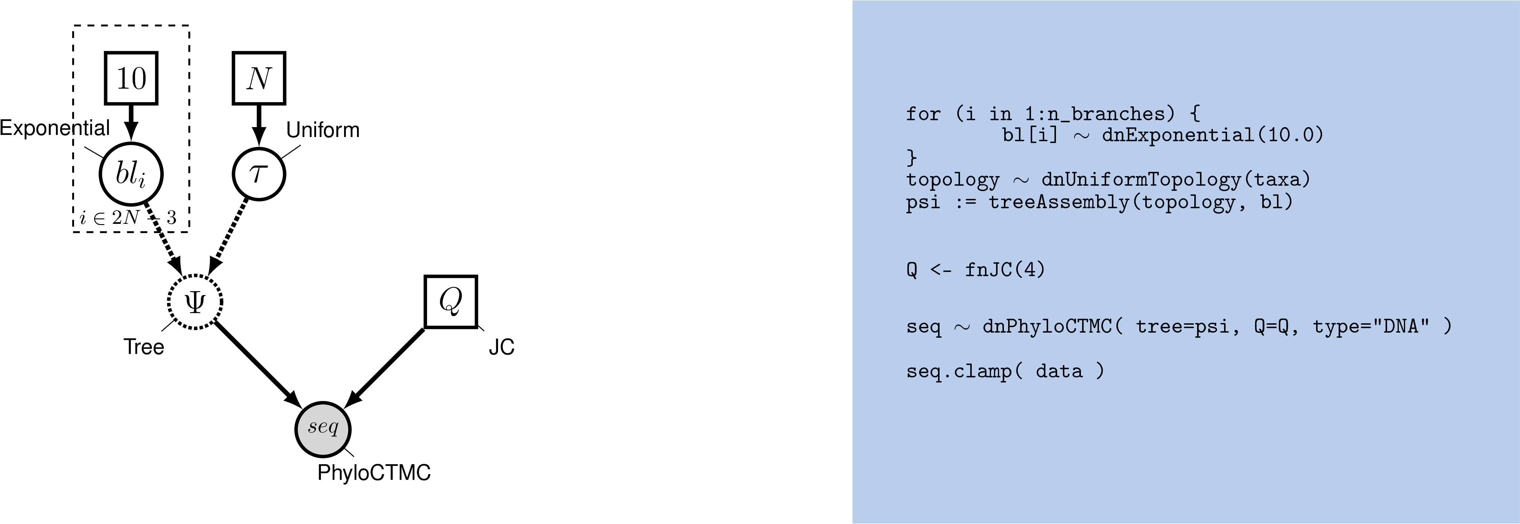
Simulating DNA sequences with an unrooted tree under the JC model requires specification of two main components: (1) the and (2) the .

Jukes-Cantor Substitution Model

A given substitution model is defined by its corresponding instantaneous-rate matrix, $Q$. The Jukes-Cantor substitution model does not have any free parameters (as the substitution rates are all assumed to be equal), so we can define it as a constant variable. The function fnJC(n) will create an instantaneous-rate matrix for a character with $n$ states. Since we use DNA data here, we create a 4x4 instantaneous-rate matrix:

Q <- fnJC(4)

• What does the “4” stand for?

You can see the rates of the $Q$ matrix by typing

Q

   [ [ -1.0000, 0.3333, 0.3333, 0.3333 ] ,
     0.3333, -1.0000, 0.3333, 0.3333 ] ,
     0.3333, 0.3333, -1.0000, 0.3333 ] ,
     0.3333, 0.3333, 0.3333, -1.0000 ] ]

As you can see, all substitution rates are equal.

Tree Topology and Branch Lengths

The tree topology and branch lengths are stochastic nodes in our phylogenetic model. In , the tree topology is denoted $\Psi$ and the length of the branch leading to node $i$ is $bl_i$.

We will assume that all possible labeled, unrooted tree topologies have equal probability. This is the dnUniformTopology() distribution in RevBayes. Note that in RevBayes it is advisable to specify the outgroup for your study system if you use an unrooted tree prior, whereas other software, such as MrBayes, use the first taxon in the data matrix file as the outgroup. Providing RevBayes with an outgroup clade will make sure that when trees are written to file, the topologies have the outgroup clade at the base, thus making the trees easier to visualize.

• Does the root position of the tree matter for the JC model?

Specify the topology stochastic node by passing in the list of taxa to the dnUniformTopology() distribution:

out_group = clade("Galeopterus_variegatus")
topology ~ dnUniformTopology(taxa, outgroup=out_group)

Next we have to create a stochastic node representing the length of each of the $2N - 3$ branches in our tree (where $N=$ n_species). We can do this using a for loop — this is a plate in our graphical model. In this loop, we can create each of the branch-length nodes. Copy this entire block of Rev code into the console:

for (i in 1:num_branches) {
   br_lens[i] ~ dnExponential(10.0)
}

Finally, we can create a phylogram (a phylogeny in which the branch lengths are proportional to the expected number of substitutions per site) by combining the tree topology and branch lengths. We do this using the treeAssembly() function, which applies the value of the $i^{th}$ member of the br_lens vector to the branch leading to the $i^{th}$ node in topology. Thus, the psi variable is a deterministic node:

psi := treeAssembly(topology, br_lens)

Alternative tree priors

For large phylogenetic trees, i.e., with more than 200 taxa, it might be more efficient to specify a combined topology and branch length prior distribution. We can achieve this by simply using the distribution dnUniformTopologyBranchLength().

br_len_lambda <- 10.0
psi ~ dnUniformTopologyBranchLength(taxa, branchLengthDistribution=dnExponential(br_len_lambda))
moves.append( mvNNI(psi, weight=num_taxa) )
moves.append( mvSPR(psi, weight=num_taxa/10.0) )
moves.append( mvBranchLengthScale(psi, weight=num_branches) )

You might think that this approach is in fact simpler than the for loop that we explained above. We thought that it was pedagogical to specify the prior on each branch length separately in this tutorial to emphasize all components of the model.

Alternative branch-length priors

Some studies, e.g. Brown et al. (2010), Rannala et al. (2012), have criticized the exponential prior distribution for branch lengths because it induces a gamma-distributed tree-length and the mean of this gamma distribution grows with the number of taxa. As an alternative, we can instead use a specific gamma prior distribution (or any other distribution yielding a positive real variable) for the tree length, and then use a Dirichlet prior distribution to break the tree length into the corresponding branch lengths (Zhang et al. 2012).

First, specify a prior distribution on the tree length with your desired mean. For example, we use a gamma distribution as our prior on the tree length.

TL ~ dnGamma(2,4)
moves.append( mvScale(TL) )

Now we create a random variable for the relative branch lengths.

rel_branch_lengths ~ dnDirichlet( rep(1.0,num_branches) )
moves.append( mvBetaSimplex(rel_branch_lengths, weight=num_branches) )
moves.append( mvDirichletSimplex(rel_branch_lengths, weight=num_branches/10.0) )

Finally, transform the relative branch lengths into actual branch lengths

br_lens := rel_branch_lengths * TL

Putting it All Together

We have fully specified all of the parameters of our phylogenetic model—the tree topology with branch lengths, and the substitution model that describes how the sequence data evolve over the tree with branch lengths. Collectively, these parameters comprise a distribution called the phylogenetic continuous-time Markov chain, and we use the dnPhyloCTMC constructor function to create this node. This distribution requires several input arguments:

1. the tree with branch lengths;
2. the instantaneous-rate matrix Q;
3. the type of character data.

Build the random variable for the character data (sequence alignment).

seq ~ dnPhyloCTMC(tree=psi, Q=Q, type="DNA", nSites=num_sites)

Simulated data

Building the seq random variable automatically simulated sequences. You can output them to a file:

writeFasta(filename="data/simulatedSequences_1.fasta", data=seq)

You can then view this alignment, for instance using seaview.

You can simulate another data set by “redrawing” the random variable:

seq.redraw()

And you can write the new sequences to another file:

writeFasta(filename="data/simulatedSequences_2.fasta", data=seq)

• Are they different from the first ones?

It is always important to evaluate the realism of simulations. In our case, we can compare the simulated alignment to the empirical alignment. The sequence data objects (“AbstractHomologousDiscreteCharacterData”) have lots of functions that we can use for this purpose:

data.methods()

Let’s use some of them to compare the empirical data to the simulated data set:

print("Mean GC content of the empirical data: " + data.meanGcContent())
print("Mean GC content of the simulated data: " + seq.meanGcContent())
print("Variance of the GC content of the empirical data: " + data.varGcContent())
print("Variance of the GC content of the simulated data: " + seq.varGcContent())

• Can you think of other statistics that might be interesting to compute to compare the empirical and the simulated data sets?

Performing inference with the JC model and the MCMC algorithm

In the first part of this tutorial, we saw how to simulate a DNA alignment using the JC model. The second part aims at performing inference under the JC model.

The inference script is called scripts/mcmc_JC.Rev. You can run it in its entirety as follows:

source("scripts/mcmc_JC.Rev")

If everything loaded properly, then you should see the program initiate the Markov chain Monte Carlo analysis that estimates the posterior distribution. If you continue to let this run, then you will see it output the states of the Markov chain once the MCMC analysis begins.

Ultimately, this is how you will execute most analyses in RevBayes, with the full specification of the model and analyses contained in the sourced files. You could easily run this entire analysis on your own data by substituting your data file name for that in the model-specification file. However, it is important to understand the components of the model to be able to take full advantage of the flexibility and richness of RevBayes. Furthermore, without inspecting the Rev scripts sourced in mcmc_JC.Rev, you may end up inadvertently performing inappropriate analyses on your dataset, which would be a waste of your time and CPU cycles. The next steps will walk you through the full specification of the model and MCMC analyses.

Additional elements in the inference script

Overall, the inference script is very similar to the simulation script. For instance, the structure of the model is the same. However, to perform inference, additional elements have to be included. In particular, the model that we were using for simulation has to be conditioned upon observed data, the sequences at the tips. Secondly, the whole model has to be assembled into a model variable, upon which MCMC sampling will be able to operate. Thirdly, moves need to be specified for each stochastic variable, so that we can obtain posterior distributions. Recall that moves are algorithms used to propose new parameter values during the MCMC simulation. Fourthly, we may want to specify monitors to record parameter values as the MCMC algorithm proceeds. Monitors print the values of model parameters to the screen and/or log files during the MCMC analysis.

Conditioning the model on observed data

The PhyloCTMC model is able to produce sequence alignments, given parameter variables. We can attach our sequence data to the tip nodes in the tree:

seq.clamp(data)

Note that although we assume that our sequence data are random variables—they are realizations of our phylogenetic model—for the purposes of inference, we assume that the sequence data are “clamped” to their observed values. When this function is called, RevBayes sets each of the stochastic nodes representing the tips of the tree to the corresponding nucleotide sequence in the alignment. This essentially tells the program that we have observed data for the sequences at the tips: we are conditioning the model on these data.

Assembling the constant, deterministic and stochastic variables into a model

We wrap the entire model in a single object to provide convenient access to the Directed Acyclic Graph. To do this, we only need to give the model() function a single node of the model. Starting from this node, the model() function can find all of the other nodes by following the arrows in the graphical model:

mymodel = model(Q)

Now we have specified a simple phylogenetic model—each parameter of the model will be estimated from every site in our alignment. If we inspect the contents of mymodel we can review all of the nodes in the DAG:

mymodel

Adding moves to the script

For each stochastic variable of the model, we need to specify a move. If no move is specified for a stochastic variable, this variable will stay constant throughout the entire algorithm.

First we create a vector to store all the moves that will be used to sample from the posterior distribution:

moves = VectorMoves()

You may have noticed that we used the = operator to create the move index. This simply means that the variable is not part of the model: it is not used to compute the probability of a set of parameter values. Instead, it is a part of the MCMC algorithm. You will later see that we use this operator for other variables that are not part of the model, e.g., when we create moves and monitors.

For instance, we specify a move for the tree topology.

moves.append( mvNNI(topology, weight=3) )

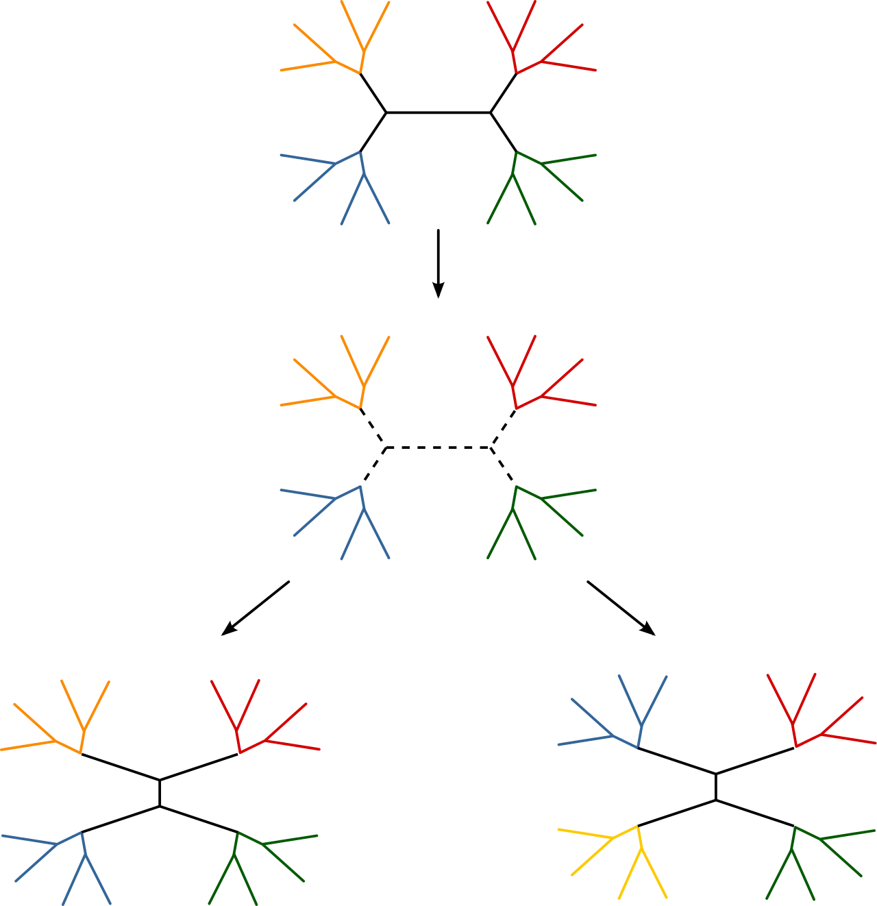
Some types of stochastic nodes, and the tree topology in particular, can be updated by a number of alternative moves. Different moves may explore parameter space in different ways, and it is possible to use multiple different moves for a given parameter to improve mixing (i.e. the efficiency of the MCMC simulation). In the case of our unrooted tree topology, for example, we can use both a nearest-neighbor interchange move (mvNNI in the Rev language) and a subtree-prune and regraft move (mvSPR in the Rev language, currently commented in the script).

These moves do not have tuning parameters associated with them, thus we only need to pass in the topology node and proposal weight.

# moves.append( mvSPR(topology, weight=3) )

The weight specifies how often the move will be applied either on average per iteration or relative to all other moves. Have a look at the MCMC tutorials for more details about moves and MCMC strategies.

The other stochastic variables in the model are branch lengths. They need their own moves:

for (i in 1:num_branches) {
    moves.append( mvScale(bl[i]) )
}

Here each branch length is associated to a mvScale move that basically multiplies the current value of a branch length by a real positive number.

• What type of stochastic variable is particularly appropriate for the mvScale move?

Specifying Monitors and Output Files

During the MCMC analysis, we can decide to keep track of all the sampled parameters, but also of various statistics that we think may be of interest. Here, we have decided to keep track of the tree length, i.e. the sum of all branch lengths. To this end, we add a variable TL that will compute this sum. Accordingly, the tree length can be computed using the sum() function, which calculates the sum of any vector of values.

TL := sum(br_lens)

• Why are we using “:=” here?

For our MCMC analysis, we need to set up a vector of monitors to record the states of our Markov chain. The monitor functions are all called mn\*, where \* is the wild-card representing the monitor type. First, we will initialize the model monitor using the mnModel function. This creates a new monitor variable that will output the states for all model parameters when passed into a MCMC function.

monitors = VectorMonitors()

monitors.append( mnModel(filename="analyses/primates_cytb_JC.log", printgen=10) )

The mnFile monitor will record the states for only the parameters passed in as arguments. We use this monitor to specify the output for our sampled phylograms.

monitors.append( mnFile(filename="analyses/primates_cytb_JC.trees", printgen=10, psi) )

Finally, we create a screen monitor that will report the states of specified variables to the screen with mnScreen:

monitors.append( mnScreen(printgen=100, TL) )

This monitor mostly helps us to see the progress of the MCMC run.

Initializing and Running the MCMC Simulation

With a fully specified model, a set of monitors, and a set of moves, we can now set up the MCMC algorithm that will sample parameter values in proportion to their posterior probability. The mcmc() function will create our MCMC object:

mymcmc = mcmc(mymodel, monitors, moves)

Now, run the MCMC:

mymcmc.run(generations=2500)

Here we set a low number of iterations. In general it is recommended to check for convergence; here it is possible that 2500 iterations may not be enough.

When the analysis is complete, you will have the files produced by the monitors in your analyses directory.

Saving and restarting analyses

MCMC analyses can take a long time to converge, and it is usually difficult to predict how many generations will be needed to obtain results. In addition, many analyses are run on computer clusters with time limits, and so may be stopped by the cluster partway through. For all of these reasons, it is useful to save the state of the chain regularly through the analysis.

mymcmc.run(generations=100000000, checkpointInterval=100, checkpointFile="analyses/primates_cytb_JC.state")

The checkpointInterval and checkpointFile inputs specify respectively how often, and to which file, the chain should be saved. Three different files will be used for storing the state: one with no extension, one with extension _mcmc, and one with extension _moves. When multiple independent runs are specified, they will automatically be saved in separate files (with extensions _run_1, _run_2, etc.).

Restarting the chain from a previous run is done by adding this line:

mymcmc.initializeFromCheckpoint("analyses/primates_cytb_JC.state")

before calling the function mcmc.run(). The file name should match what was given as checkpointFile when running the previous analysis. NB: Note that this line will create an error if the state file does not exist yet, and so should be commented out in the first run.

The full MCMC block thus becomes:

mymcmc = mcmc(mymodel, monitors, moves, nruns=1)
mymcmc.initializeFromCheckpoint("analyses/primates_cytb_JC.state") #comment this out for the first run

mymcmc.run(generations=100000000, checkpointInterval=100, checkpointFile="analyses/primates_cytb_JC.state")

Summarizing MCMC Samples

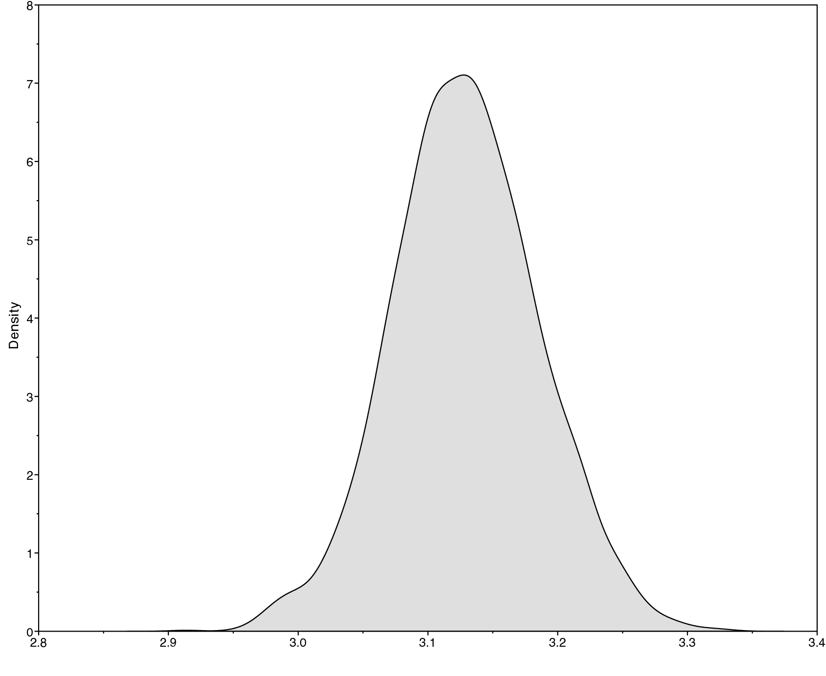
Methods for visualizing the marginal densities of parameter values are not currently available in RevBayes itself. Thus, it is important to use programs like Tracer (Rambaut and Drummond 2011) to evaluate mixing and non-convergence.

Look at the file called analyses/primates_cytb_JC.log in Tracer. There you see the posterior distribution of the continuous parameters, e.g., the tree length variable TL.

It is always important to carefully assess the MCMC samples for the various parameters in your analysis. You can read more about MCMC tuning and evaluating and improving mixing in the other tutorials on the RevBayes website.

Analyzing the inferred phylogeny

We are interested in the phylogenetic relationship of the Tarsiers. Therefore, we need to summarize the trees sampled from the posterior distribution. RevBayes can summarize the sampled trees by reading in the tree-trace file:

treetrace = readTreeTrace("analyses/primates_cytb_JC.trees", treetype="non-clock")

The mapTree() function will summarize the tree samples and write the maximum a posteriori tree to file:

map_tree = mapTree(treetrace,"analyses/primates_cytb_JC_MAP.tree")

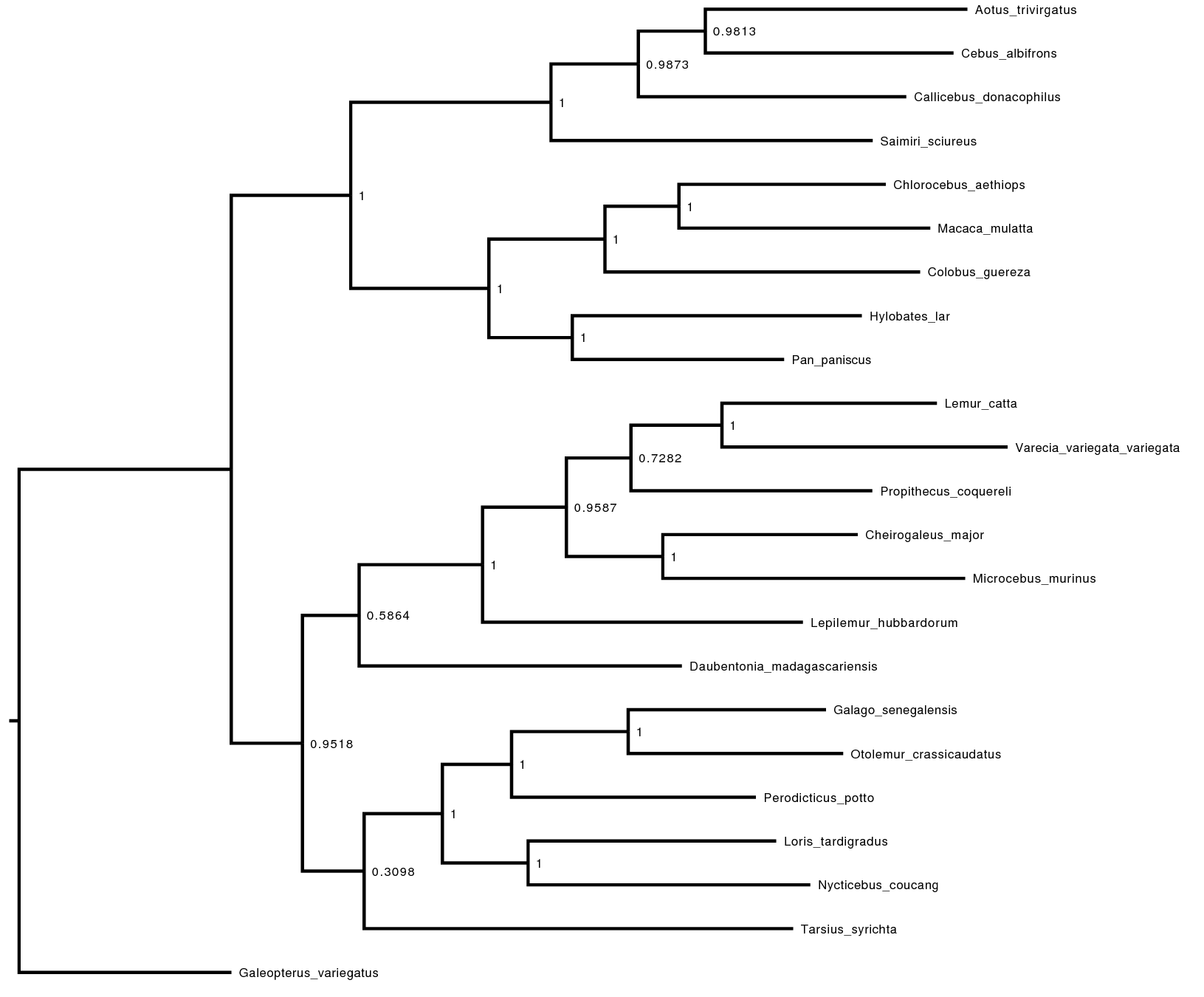
Look at the file called analyses/primates_cytb_JC_MAP.tree in FigTree. We show it in .

Note, you can query the posterior probability of a particular clade being monophyletic using the following command:

Lemuroidea <- clade("Cheirogaleus_major",
                    "Daubentonia_madagascariensis",
                    "Lemur_catta",
                    "Lepilemur_hubbardorum",
                    "Microcebus_murinus",
                    "Propithecus_coquereli",
                    "Varecia_variegata_variegata")

treetrace.cladeProbability( Lemuroidea )

Conclusion

During this tutorial, we used the simplest phylogenetic model to first simulate data, and then infer a phylogeny given an empirical data set. Sequence simulation is often used to test inference methods.

• What could you learn by performing MCMC inference on a simulated data set?
• Combine the scripts to perform inference on simulated data.

Sequence simulation is also often used to assess model adequacy, i.e. to ask if my model can reproduce the important features of the empirical data set.

• Based on a comparison of the empirical and simulated alignments, do you think that the JC model is adequate for this data set?

In the next tutorial, you will learn about more sophisticated models of sequence evolution.

1. Brown J.M., Hedtke S.M., Lemmon A.R., Lemmon E.M. 2010. When Trees Grow Too Long: Investigating the Causes of Highly Inaccurate Bayesian Branch-Length Estimates. Systematic Biology. 59:145–161. 10.1093/sysbio/syp081
2. Höhna S., Heath T.A., Boussau B., Landis M.J., Ronquist F., Huelsenbeck J.P. 2014. Probabilistic Graphical Model Representation in Phylogenetics. Systematic Biology. 63:753–771. 10.1093/sysbio/syu039
3. Jukes T.H., Cantor C.R. 1969. Evolution of Protein Molecules. Mammalian Protein Metabolism. 3:21–132. 10.1016/B978-1-4832-3211-9.50009-7
4. Rambaut A., Drummond A.J. 2011. Tracer v1.5. . http://tree.bio.ed.ac.uk/software/tracer/
5. Rannala B., Zhu T., Yang Z. 2012. Tail Paradox, Partial Identifiability, and Influential Priors in Bayesian Branch Length Inference. Molecular Biology and Evolution. 29:325–335.
6. Zhang C., Rannala B., Yang Z. 2012. Robustness of Compound Dirichlet Priors for Bayesian Inference of Branch Lengths. Systematic Biology. 61:779–784.