Thus far, the phylogenetic analyses have been conducted in an undated context: the tree was not ultrametric (i.e. was not a dated tree). Instead, the branch lengths were measured directly in expected numbers of substitutions per site (i.e. sequence divergence, not absolute nor even relative time).
In this tutorial, we will do dated analyses. However, we will not use fossil calibrations, which introduce some complications (but if you want to set up a fossil calibration see the end of the tutorial). As a result, the dates will be relative (arbitrarily, the age of the root is equal to 1, and all other dates are thus between 0 and 1). We will explore two alternative clock models, with a third optional one:
a strict molecular clock
a non auto-correlated clock: each branch has an independent rate
an auto-correlated clock: the substitution rate on a branch tends to be similar to the rate of the neighbouring branches
All analyses will be done under a fixed tree topology. This topology has been estimated by using an undated model, such as seen during the previous tutorials.
Take a look at the tree data/prim.tree using software like FigTree. Is this tree ultrametric? Which lineages seem to have been associated with a high rate of molecular evolution?
We will work on a dataset (file name prim4fold.nex) with 58 primates species, plus 2 Dermopterans and a Scandentia (Tupaia), which will be our outgroup. The dataset is adapted from Perelman et al (2011, PLoS Genetics, 7:e1001342, A Molecular Phylogeny of Primates). Here, we use only the 4-fold degenerate third coding positions (1730 aligned nucleotide positions).
Strict clock model
To start the tutorial, we give a script (prim_strictclock.rev), which implements the strict clock model.
The script is set up as follows.
We first read the nucleotide sequence alignment and get the taxon set and the number of species and the number of branches.
Why is the number of branches 2 * n_species - 2 and not 2 * n_species - 3 as in the undated case?
Next, we define our dated tree. We first need to create a variable standing for the age of the root:
root_age ~ dnUniform(0,100)
This root age will be fixed (see below). However, we still need to specify it as a random variable.
Then, we assume that the tree is produced by a birth-death process, with unknown speciation and extinction rates equal to lambda and mu. We also assume that a fraction rho of all extant species are present in our dataset, and that these species have been randomly sampled among all extant species:
# speciation rate
lambda ~ dnUniform(0.0, 10)
# extinction rate
mu ~ dnUniform(0.0, 10)
# sampling fraction (in the present)
# here, we assume that we have sampled 20% of the species in our clade
rho <- 0.2

# time tree produced by a birth-death process (BDP)
timetree ~ dnBDP(lambda, mu, rho, root_age, samplingStrategy="uniform", condition="nTaxa", taxa=taxa)
Next, we want to fix the tree topology, setting it equal to the topology given in the file named prim.tree:
# read tree from file
tree <- readTrees("data/prim.tree", treetype="clock")[1]
# adjust terminal branch lengths so as to make the tree ultrametric
tree.makeUltrametric()

# set the value of the tree topology
timetree.setValue(tree)
The tree given in this file has an arbitrary root age. We rescale it, setting it equal to 1.0:
# rescale root age to 1.0
# (all ages will be relative to the root)
root_age.setValue(1.0)
Altogether, we have specified a constrained dated tree, whose topology is fixed, and whose root is constrained to be at age $1.0$. On the other hand, the ages of the nodes will still be allowed to vary. These node ages will be determined by a compromise between the birth-death (or constant speciation-extinction) process, which is used here as a prior on divergence times, and the information obtained from the nucleotide sequences.
Now that we have a tree, we can model the process of substitution along this tree. We first have to specify the absolute substitution rate (the speed of the molecular clock). This rate is unknown, so we will put a prior on it, which we want to be uninformative. Here, we use an exponential prior of mean 1:
# we assume a strict molecular clock, of unknown rate
clockrate ~ dnUniform(0.0,10.0)
Of note, a rough estimate of the age of primates is between 50 and 100 Myr, and the mutation rate per year in Humans is of the order of $10^{-9}$ per year, which gives us a rough estimate of $\sim 10^{-1}$ substitution over the total time span of the tree (100 Myr). Thus, our uniform prior on the rate of sequence evolution should be safe.
Then, we specify the Tamura 92 nucleotide substitution process:
# and a T92 process
kappa ~ dnUniform(0.0,10.0)
gamma ~ dnBeta(1.0, 1.0)
Q := fnT92(kappa=kappa, gc=gamma)
Note that we have no move on the tree topology (since we want to fix the topology).
For the monitoring streams, we can record the parameters and the trees, while printing the clock rate, the transition-transversion ratio and the equilibrium GC content onto screen:
Once the analysis has run, first, we can estimate the burn-in and obtain a point estimate and a credible interval for the clock rate, using Tracer.
Next, we can read the tree trace and make the MAP tree:
Of note, this MAP tree will, by construction, have the same topology as the one given at the beginning of the script. The point of doing this map tree is just to have credible intervals on the node ages.
The resulting tree, saved into the file named prim_strictclock.tree, can be visualized using FigTree. The credible intervals on node ages can be visualized as blue bars attached to the corresponding nodes.
Run the script on the primate dataset. Estimate the clock rate (median and credible interval) and visualize the estimated relative ages.
The non auto-correlated relaxed clock model
The model considered in the previous section assumes that the rate of evolution does not vary through time. In practice, this assumption is generally violated, and this can result in important biases in date estimation. Therefore, we need to account for variation in the substitution rate across the tree.
A first model, often used in the recent literature, is the non auto-correlated model. This model assumes that each branch has its own rate of substitution. The rates across branches are independent and identically distributed. They can be either exponential, gamma or log-normal. In the following, we will consider a gamma model: branch rates are i.i.d. gamma. The mean and the variance of this gamma distribution are unknown and should therefore be estimated – as always, by specifying them as random variables with a prior.
To implement this model, we start by specifying the mean and the variance of the rate of sequence evolution. Here, we will parameterize the model in terms of the mean rate and the relative variance, or coefficient of variation (variance divided by the square of the mean). This parameterization is more convenient. In both cases, we use a uniform prior:
Next, we need to express the shape and the scale parameter of the gamma distribution as functions of the mean and the relative variance. Remember that, for a gamma distribution of shape parameter $\alpha$ and scale parameter $\beta$, the mean $m$ and the variance $v$ of the distribution are given by $m = \alpha / \beta$ and $v = \alpha / \beta^2$. Therefore, the relative variance $c$ is equal to $c = v / m^2 = 1.0 / \alpha$.
Inverting these relations allows us to express $\alpha$ and $\beta$ as a function of $m$ and $c$ as follows: $\alpha = 1 / c$ and $\beta = \alpha / m$. In the context of our script, this gives:
Note that clockrate is now a vector (whereas, in the case of the strict clock model considered in the last section, it was a scalar). When receiving a vector, the dnPhyloCTMC object automatically deduces that the rates in the vector should be mapped onto the branches of the tree.
For the rest, the script is essentially the same as for the strict clock model considered above. The main difference is that moves should now be implemented for mean_clockrate, relvar_clockrate, and for each of the entries of the clockrate vector. Implementing these moves is left as an exercise.
Write the complete script, using prim_strictclock.rev as a template and making the required changes. You may want to remove the variable clockrate from the screen monitor to avoid cluttering your terminal, and instead you may want to monitor mean_clockrate. Run the script on the primate dataset. Estimate the mean rate of substitution and its relative variance across branches. Visualize the estimated relative ages on the tree.
How does this compare with the strict clock estimates?
Using FigTree, identify areas of high or low rates of evolution.
How does this compare to the fast- or slow-evolving lineages identified by looking at the undated tree?
The auto-correlated relaxed clock model
The non auto-correlated model is convenient and easy to implement. However, empirically, it is not so adequate. The main reason is that the rate of evolution tends to show strong auto-correlation between neighbouring branches. Just think, for instance, that the rate of evolution is partly determined by the generation time (species with longer generation times tend to be more slowly evolving). Yet closely related species tend to have similar generation times. In other words, the generation time (and therefore the substitution rate) shows phylogenetic inertia.
One way to account for this auto-correlation is to assume that the logarithm of the substitution rate evolves along the tree according to a Brownian model. This idea has been implemented in several software programs, such as MultiDivTime, PhyloBayes or Coevol.
Specifically, consider a trait $X$, evolving according to a Brownian process, with variance $\sigma^2$ per unit of time. This means that, given the value of the trait at some time $t$, $X(t)$, then, the value of the trait at time $t+\Delta t$ is normally distributed, of mean $X(t)$ and of variance $\sigma^2 \Delta t$:
\[X(t + \Delta t) \sim Normal \left( X(t), \sigma^2 \Delta t \right)\]
We can use this equation to model the distribution of the substitution rates at the nodes of the tree: consider some node $n$ of the tree, other than the root, and which lives at time $u$. Consider the node immediately before node $n$ (the parent of $n$), and call it $m$. Node $m$ lives at time $t < u$. Let $X(t)$ denote the log of the rate at node $m$. Then, according to the equation above, $X(u)$ is normally distributed, as follows:
\(X(u) \sim Normal(X(t), \sigma^2 (t-u))\)
Note that $t-u$ is just the length of the branch starting at node $m$ and ending at node $n$.
With this equation, we can define the log of the substitution rate (or, more briefly, log-rate) at each node (other than the root) as a normally-distributed random variable, whose distribution depends on the log-rate of the parent node. The exception is the root node, which does not have a parent. So, we need to define a prior distribution for the value of the log of the substitution rate at the root.
In practice, we need to proceed in the other direction: first specifying the log-rate at the root, then, going from the root to the tips of the tree, and specifying the distribution of the log-rate at each node, conditional on its parent. In RevBayes, the nodes are indexed starting from the tips, and ending at the root. Therefore, we should specify them by visiting the indices in a decreasing order.
First, we define the number of nodes:
n_nodes <- 2 * n_species - 1
Then we should define the sigma parameter (the variance per unit of time of the Brownian motion):
sigma ~ dnExponential(1.0)
Next, we should specify the log-rate at the root, which has index n_nodes. Here, we use a vaguely informative prior, with a rate of mean around $0.1$, but with a large variance:
nodelograte[n_nodes] ~ dnNormal(mean=-2, sd=20)
Then, we visit the nodes in decreasing order (from root to tips):
for (i in (n_nodes-1):1)    {
    nodelograte[i] ~ dnNormal(mean=nodelograte[tree.parent(i)], sd=sigma * sqrt(tree.branchLength(i)))
}
Once this is done, we still need to specify (or, in fact, to approximate), the mean substitution rate over each branch. We will use the following approximation: the rate on a given branch is the average of the rates at both ends. The rates at both ends are themselves obtained by taking the exponential of the log-rates at both ends. Altogether, we have to loop over all branches as follows:
for (i in 1:n_branches) {
    clockrate[i] := 0.5 * (exp(nodelograte[tree.parent(i)]) + exp(nodelograte[i]))
}
Finally, we can use these rates across branches in our sequence evolutionary process:
Again, we should move all of the additional free parameters of the model: here, a scaling move for sigma:
moves.append(mvScale(sigma, weight=1.0))
but also a sliding move for each of the log-rates across nodes.
for (i in 1:n_nodes) {
    moves.append(mvSlide(nodelograte[i], weight=1.0))
}
For the rest, the script unfolds as usual.
Write the complete script, using prim_strictclock.rev as a template and making the required changes. Run the script on the primate dataset, and compare your estimation with the other clock models considered above.
Setting up a node age calibration
To date a phylogeny it is useful to be able to associate a date in time to one or several nodes (i.e., clades) of the phylogeny. This is called calibrating a node age. Typically, node age calibrations can be obtained from the fossil record. In this primate phylogeny, several fossils could be used to calibrate the age of several nodes. Here we will calibrate a single node in the phylogeny, but in practice it is often better to calibrate several nodes using several fossil ages.
We will calibrate the node ancestral to all Anthropoidea. To do this, we first need to define the corresponding clade:
From the literature we find that it can be calibrated with a minimum age at 31.5 Mya. We will implement this calibration as a minimum bound, which means that we assume that the clade was formed before that time.
minimum_bound_Anthropoidea <- 31.5
Then, we compute the clade age (i.e., the time at which the clade was born) as found in the timetree in the current iteration of the MCMC:
Finally we calibrate the node age with the fossil age. Because we are using a minimal bound, we know that the node age has to be older than the fossil age. The delay between the node age and the fossil age is considered to be distributed according to an exponential distribution. However the writing of this simple assumption is a bit tricky: we are going to write that the variable that is clamped is generated according to an exponential waiting time that started at time -speciation_clade_Anthropoidea. Here is how we specify this:
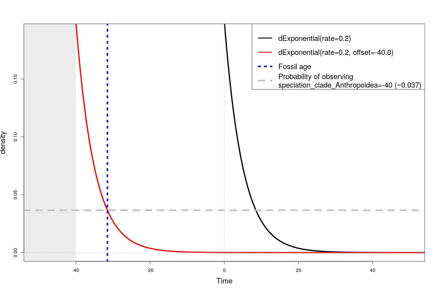
The figure below shows how a common exponential distribution (in black) shifts when it is offset by a value of -40 (i.e., here speciation_clade_Anthropoidea=40). According to this shifted distribution, the likelihood of observing the fossil at age -31.5 is about 0.037.
Density of an exponential distribution without and with offset, and the likelihood of observing fossil age -31.5 given clade age -40.
One way to interpret this calibration is to represent the likelihood for different values of the clade age speciation_clade_Anthropoidea. This is shown in the figure below.
Likelihood curve for clade age speciation_clade_Anthropoidea given fossil age -31.5 and rate for the exponential distribution 0.2.
We observe that the most likely clade ages are right before the fossil age, and that the likelihood of clade age decreases as the clade becomes much older than the fossil age.
Finally, implementing this node age calibration into the relaxed clock scripts involves copying the code lines given above, but also changing how we handle the root age, which we had fixed to be 1.0 (we were using root_age.setValue(1.0), we need to remove this line). Instead, we need to sample root age values by specifying moves on the root age, as follows: